Statistics for Python

1 Introduction

Statistics for Python is an extension module, written in ANSI-C, for the Python scripting language. Currently, this extension module contains some routines to estimate the probability density function from a set of random variables.
Statistics for Python was released under the Python License.
Michiel de Hoon
Center for Computational Biology and Bioinformatics, Columbia University.

2 Descriptive statistics

Statistics for Python currently contains four functions for descriptive statistics: The mean, the median, the Pearson correlation, and a function to fit a linear regression line.

2.1 Univariate descriptive statistics

B. P. Welford: “Note on a method for calculating corrected sums of squares and products.” Technometrics 4(3): 419-420 (1962).
Peter M. Neely: “Comparison of several algorithms for computation of means, standard deviations and correlation coefficients.” Communications of the ACM 9(7): 496-499 (1966).
The arithmetic mean is defined as

\overline{x} = \frac{1}{n} \sum_{i = 1}^{n} x_{i}

The statistical median of the data

x_{i}

is defined as

\tilde{x} = {x'}_{(n + 1) / 2} n is odd \frac{1}{2} ({x'}_{n / 2} + {x'}_{1 + n / 2}) n is even

where we find the array

x'

by sorting the array

x .

The variance in a random variable

x

is defined as

σ_{x}^{2} = E [{(x - E (x))}^{2}]

Given

n

data of

x,

the unbiased estimate of the variance is

{\hat{σ}}_{x}^{2} = \frac{1}{n - 1} [(\sum_{i = 1}^{n} x_{i}^{2}) - \frac{1}{n} {(\sum_{i = 1}^{n} x_{i})}^{2}] .

For the maximum-likelihood estimate of the variance, which is a biased estimate, we divide by

n

instead of

n - 1 .

The variance in this library is implemented using the algorithm proposed by Welford (1962), which avoids the round-off errors associated with a direct calculation of the variance.

2.2 Multivariate descriptive statistics

Ronald A. Fisher: “Statistical Methods for Research Workers”, chapter VII. Oliver and Boyd, Edinburgh/London (1925).”

2.2.1 Covariance

The covariance between two random variables

x

and

y

is defined as

σ_{x y} = E [(x - E (x)) (y - E (y))]

Given

n

paired data of

x

and

y,

the unbiased estimate of their covariance is

{\hat{σ}}_{x y} = \frac{1}{n - 1} [(\sum_{i = 1}^{n} x_{i} y_{i}) - \frac{1}{n} (\sum_{i = 1}^{n} x_{i}) (\sum_{i = 1}^{n} y_{i})];

for the maximum-likelihood estimate of the covariance, which is a biased estimate, we divide by

n

instead of

n - 1 .

The covariance is calculated using the algorithm proposed by Welford (1962) to avoid round-off errors.

2.2.2 Correlation

Statistics for Python includes the following correlation measures:

Pearson correlation
Spearman rank correlation
Intraclass correlation

The Pearson correlation is calculated using the algorithm proposed by Welford (1962) to avoid round-off errors. The intraclass correlation follows the definition by Fisher: in which To avoid round-off error, the intraclass correlation is calculated using a recursion formula similar to the Welford algorithm: in which are calculated from the recursion formulae with

2.2.3 Linear regression

Calculate the intercept and slope of a linear regression line through a cloud of points.

2.3 Usage

2.3.1 Mean

The function mean returns the arithmetic mean of an array of data.
>>> mean(x)

Arguments

Return values

The arithmetic mean of the data x.

2.3.2 Median

The function median returns the median of an array of data.
>>> median(x)

Arguments

Return values

The median of the data x.

2.3.3 Variance

The function variance calculates the variance of a one-dimensional array of data.
>>> variance(x, mode = "Unbiased")

Arguments

x
mode

mode

Unbiased

variance

mode

ML

Return values

The variance in x.

2.3.4 Covariance

The function covariance calculates the covariance matrix of an array of data.
>>> covariance(x, y = None, mode = "Unbiased")

Arguments

If x is a one-dimensional array and y==None, then this function returns the variance of x;
If both x and y are one-dimensional arrays with the same length, covariance returns the covariance between x and y;
If x is a two-dimensional array, then covariance returns the covariance matrix of x; y is ignored.

x

None

mode

mode

Unbiased

covariance

mode

ML

Return values

If x is one-dimensional and y==None: the variance in x;
If x and y are both one-dimensional and have the same length: the covariance between x and y;
If x is two-dimensional: the covariance matrix between the columns of x. Element [i,j] of the covariance matrix contains the covariance between columns x[:,i] and x[:,j].

2.3.5 Correlation

The function correlation calculates the correlation matrix of an array of data.
>>> correlation(x, y = None, method = "Pearson")

Arguments

If x is a one-dimensional array and y==None, then this function returns 1.0;
If both x and y are one-dimensional arrays with the same length, correlation returns the correlation between x and y;
If x is a two-dimensional array, then correlation returns the correlation matrix of x; y is ignored.

x

None

method

"Pearson": The Pearson correlation (default);
"Spearman": The Spearman rank correlation;
"Intraclass": The intraclass correlation.

Return values

If x is one-dimensional and y==None: 1.0;
If x and y are both one-dimensional and have the same length: the correlation between x and y;
If x is two-dimensional: the correlation matrix between the columns of x. Element [i,j] of the correlation matrix contains the correlation between columns x[:,i] and x[:,j].

2.3.6 Linear regression

The function regression returns the intercept and slope of a linear regression line fit to two arrays x and y.
>>> a, b = regression(x,y)

Arguments

The size of x and y should be equal.

Return values

3 Kernel estimation of probability density functions

B. W. Silverman: “Density Estimation for Statistics and Data Analysis”, Chapter 3. Chapman and Hall, New York, 1986.
D. W. Scott: “Multivariate Density Estimation; Theory, Practice, and Visualization”, Chapter 6. John Wiley and Sons, New York, 1992.

Suppose we have a set of observations

x_{i}

, and we want to find the probability density function of the distribution from which these data were drawn. In parametric density estimations, we choose some distribution (such as the normal distribution or the extreme value distribution) and estimate the values of the parameters appearing in these functions from the observed data. However, often the functional form of the true density function is not known. In this case, the probability density function can be estimated non-parametrically by using a kernel density estimation.

3.1 Kernel estimation of the density function

Histograms are commonly used to represent a statistical distribution. To calculate a histogram, we divide the data into bins of size

2 h

, and count the number of data in each bin. Formally, we can write this as

\hat{f} (x) = \frac{1}{n h} \sum_{i = 1}^{n} k (\frac{x - x_{i}}{h})

where the function

k

is defined by

k t \frac{1}{2} x 1 0 x 1

and

h

is called the bandwidth, smoothing parameter, or window width. Here, the probability density is estimated for a given value of

x

which corresponds to the center of each bin in the histogram. More generally, by varying

x

we can estimate the probability density function

f (x)

as a function of

x

. Using the kernel function

k

as defined above yields the naïve estimator of the probability density function. As the kernel function is not continuous, the naïve estimator tends to produce jagged probability density functions. Hence, we replace the flat-top kernel function by some smooth (and usually symmetric and non-negative) function. In order to guarantee that the estimated density function integrates to unity, we also require

t k t 1

Some commonly used kernel functions are listed in the table below. The Epanechnikov kernel is used by default, as it can (theoretically) minimize the mean integrated square error of the estimation. In practice, there is little difference in the integrated square error between probability density functions estimated with different kernels, and it may be worthwhile to choose a different kernel based on other considerations, such as differentiability.

Mnemonic	Kernel name	Function	Optimal bandwidth $h$
`'u'`	Uniform	$k t \frac{1}{2} t 1 0 t 1$	$σ {(\frac{12 \sqrt{π}}{n})}^{\frac{1}{5}}$
`'t'`	Triangle	$k t 1 t t 1 0 t 1$	$σ {(\frac{64 \sqrt{π}}{n})}^{\frac{1}{5}}$
`'e'`	Epanechnikov	$k t \frac{3}{4} (1 - t^{2}) t 1 0 t 1$	$σ {(\frac{40 \sqrt{π}}{n})}^{\frac{1}{5}}$
`'b'`	Biweight/quartic	$k t \frac{15}{16} {(1 - t^{2})}^{2} t 1 0 t 1$	$σ {(\frac{280 \sqrt{π}}{3 n})}^{\frac{1}{5}}$
`'3'`	Triweight	$k t \frac{35}{32} {(1 - t^{2})}^{3} t 1 0 t 1$	$σ {(\frac{25200 \sqrt{π}}{143 n})}^{\frac{1}{5}}$
`'c'`	Cosine	$k t \frac{π}{4} cos \frac{π}{2} t t 1 0 t 1$	$σ {(\frac{π^{\frac{13}{2}}}{6 n {(π^{2} - 8)}^{2}})}^{\frac{1}{5}}$
`'g'`	Gaussian	$k t \frac{1}{\sqrt{2 π}} exp (- \frac{1}{2} t^{2})$	$σ {(\frac{4}{3 n})}^{\frac{1}{5}}$

Estimating the probability density function with the Gaussian kernel is more computationally intensive than with other kernels, as it has infinite support (i.e.,

k (t)

is nonzero for all

t

3.2 Kernel estimation of the cumulative probability density

By integrating the estimated probability density function, we obtain an estimate for the cumulative density function

F (x)

\hat{F} (x) = t x \hat{f} (t) = \frac{1}{n} \sum_{i = 1}^{n} K (\frac{x - x_{i}}{h}),

where

K

is defined as the primitive of the kernel function

k

K (x) \equiv t x k (t)

This software package contains a Python function to calculate this estimate directly from a set of data, as well as a function to estimate the complementary cumulative probability density, defined as

F^{'} (x) \equiv 1 - F (x)

The complementary cumulative probability density

F^{'} (x)

can be interpreted as the tail probability

p

of the random variable to be equal to or larger than

x

assuming that it is drawn from the distribution described by

f

3.3 Choosing the bandwidth

The bandwidth

h

determines how smooth the estimated probability density function will be: A larger value for

h

leads to a smoother probability density function, as it is averaged over more data points. Often, a suitable bandwith can be chosen subjectively based on the application at hand. Alternatively, we may choose the bandwidth such that it minimizes the asymptotic mean integrated square error. This optimal bandwidth depends on the number of observations

n

, the standard deviation

σ

of the observed data, and the kernel function. The formulas for the optimal bandwidth are given in the table above. To make things easy, this software package contains a Python function to calculate the optimal bandwidth from the data.

3.4 Usage

3.4.1 Estimating the probability density function

The function pdf estimates the probability density function from the observed data. You can either specify the values of x at which you want to estimate the value y of the probability density function explicitly:
>>> y = pdf(data, x, weight = None, h = None, kernel = 'Epanechnikov')
or you can let the function choose x for you:
>>> y, x = pdf(data, weight = None, h = None, kernel = 'Epanechnikov', n = 100)
In the latter case, the returned array x contains n equidistant data points covering the domain where

\hat{f} (x)

is nonzero.

Arguments

data
weight

weight==None

x

pdf

x

n

h

bandwidth

kernel

'E' or 'Epanechnikov': Epanechnikov kernel (default)
'U' or 'Uniform': Uniform kernel
'T' or 'Triangle': Triangle kernel
'G' or 'Gaussian': Gaussian kernel
'B' or 'Biweight': Quartic/biweight kernel
'3' or 'Triweight': Triweight kernel
'C' or 'Cosine': Cosine kernel

x

n

Return values

If you specified x explicitly: The estimated probability density, estimated at at the values in x;
If you did not specify x explicitly: The estimated probability density, as well as the corresponding values of x.

3.4.2 Estimating the cumulative probability density function

The function cpdf estimates the cumulative probability density function from the observed data. You can either specify the values of x at which you want to estimate the value y of the cumulative probability density function explicitly:
>>> y = cpdf(data, x, h = None, kernel = 'Epanechnikov')
or you can let the function choose x for you:
>>> y, x = cpdf(data, h = None, kernel = 'Epanechnikov', n = 100)
In the latter case, the returned array x contains n equidistant data points covering the domain where

\hat{f} (x)

is nonzero; the estimated cumulative probability density is constant (either 0 or 1) outside of this domain.

Arguments

data
x

x

cpdf

x

n

h

bandwidth

kernel

'E' or 'Epanechnikov': Epanechnikov kernel (default)
'U' or 'Uniform': Uniform kernel
'T' or 'Triangle': Triangle kernel
'G' or 'Gaussian': Gaussian kernel
'B' or 'Biweight': Quartic/biweight kernel
'3' or 'Triweight': Triweight kernel
'C' or 'Cosine': Cosine kernel

x

n

Return values

If you specified x explicitly: The estimated cumulative probability density, estimated at at the values in x;
If you did not specify x explicitly: The estimated cumulative probability density, as well as the corresponding values of x.

3.4.3 Estimating the complement of the cumulative probability density function

The function cpdfc estimates the complement of the cumulative probability density function from the observed data. You can either specify the values of x at which you want to estimate the value y of the complement of the cumulative probability density function explicitly:
>>> y = cpdfc(data, x, h = None, kernel = 'Epanechnikov')
or you can let the function choose x for you:
>>> y, x = cpdfc(data, h = None, kernel = 'Epanechnikov', n = 100)
In the latter case, the returned array x contains n equidistant data points covering the domain where

\hat{f} (x)

is nonzero; the estimated complement of the cumulative probability density is constant (either 0 or 1) outside of this domain.

Arguments

data
x

x

cpdfc

x

n

h

bandwidth

kernel

'E' or 'Epanechnikov': Epanechnikov kernel (default)
'U' or 'Uniform': Uniform kernel
'T' or 'Triangle': Triangle kernel
'G' or 'Gaussian': Gaussian kernel
'B' or 'Biweight': Quartic/biweight kernel
'3' or 'Triweight': Triweight kernel
'C' or 'Cosine': Cosine kernel

x

n

Return values

If you specified x explicitly: The estimated cumulative probability density, estimated at at the values in x;
If you did not specify x explicitly: The estimated cumulative probability density, as well as the corresponding values of x.

3.4.4 Calculating the optimal bandwidth

The function bandwidth calculates the optimal bandwidth from the observed data for a given kernel:
>>> h = bandwidth(data, weight=None, kernel='Epanechnikov')

Arguments

data
weight

weight==None

kernel

'E' or 'Epanechnikov': Epanechnikov kernel (default)
'U' or 'Uniform': Uniform kernel
'T' or 'Triangle': Triangle kernel
'G' or 'Gaussian': Gaussian kernel
'B' or 'Biweight': Quartic/biweight kernel
'3' or 'Triweight': Triweight kernel
'C' or 'Cosine': Cosine kernel

Return value

The function bandwidth returns the optimal bandwidth for the given data, using the specified kernel. This bandwidth can subsequently be used when estimating the (cumulative) probability density with pdf, cpdf, or cpdfc.

3.5 Examples

3.5.1 Estimating a probability density function

We use Numerical Python's random module to draw 100 random numbers from a standard normal distribution.
>>> from numpy.random import standard_normal
>>> data = standard_normal(100)
We estimate the probability density function, using the default Epanechnikov kernel and the default value for the bandwidth:
>>> import statistics
>>> y, x = statistics.pdf(data)
The estimated probability function y as a function of x is drawn below (figure created by Pygist).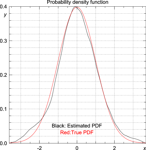

Similarly, we can estimate the cumulative probability density distribution:
>>> y, x = statistics.pdf(data)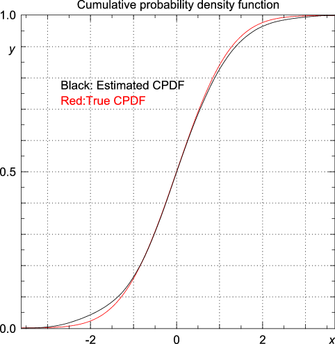

3.5.2 Choosing the kernel and bandwidth

We now use Numerical Python's random module to generate 20000 random numbers from a distribution consisting of two Gaussians, one centered around -3 and one centered around 3, both with a standard deviation equal to unity.
>>> from numpy.random import standard_normal, randint
>>> n = 20000
>>> data = standard_normal(n) + 3.0*(randint(0,2,n)-0.5)
Next, we estimate the probability density function, using the Epanechnikov kernel and the default value for the bandwidth:
>>> import statistics
>>> y, x = statistics.pdf(data)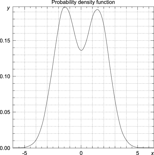

The choice of kernel function usually has a minor effect on the estimated probability density function:
>>> y, x = statistics.pdf(data, kernel="Gaussian")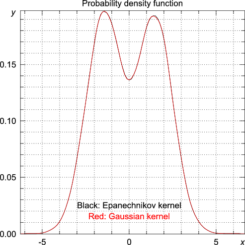

Now, let's find out the default value for the bandwidth was:
>>> statistics.bandwidth(data)
0.58133427540755089
Choosing a bandwidth much smaller than the default value results in overfitting:
>>> y, x = statistics.pdf(data, h = 0.58133427540755089/10)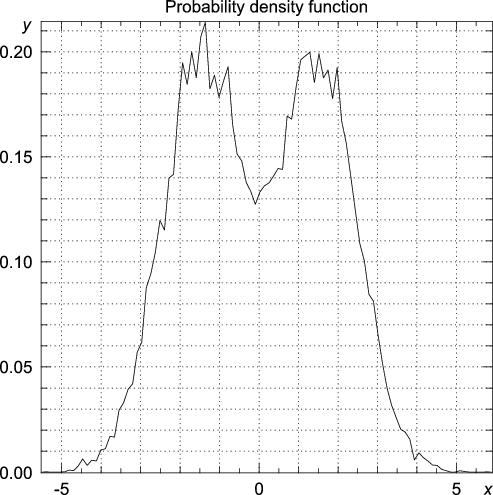

Choosing a bandwidth much larger than the default value results in oversmoothing:
>>> y, x = statistics.pdf(data, h = 0.58133427540755089*4)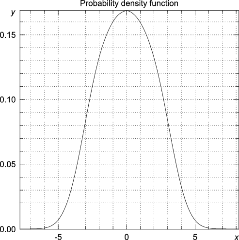

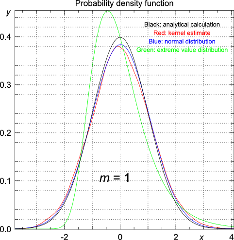
3.5.3 Approaching the extreme value distribution

Suppose we generate

m

random numbers

u

from a standard normal distribution, and define

x

the maximum of these

m

numbers. By repeating this

n

times, we obtain

n

random numbers whose distribution, for

m

large, approaches the extreme value distribution. Given that the random numbers

u

are drawn from a standard normal distribution, we can calculate the distribution of

x

analytically:

f_{m} (x) = \frac{m}{\sqrt{2 π}} {(\frac{1}{2} - \frac{1}{2} erf (\frac{x}{\sqrt{2}}))}^{m - 1} exp (- \frac{x^{2}}{2})

However, in general the distribution of

u

, and therefore

x

, is unknown, except that for

m

large we can approximate the distribution of

x

by an extreme value distribution:

f_{a, b} (x) = \frac{1}{b} exp (\frac{a - x}{b} - exp (\frac{a - x}{b})),

where

a

and

b

are estimated from the mean and variance of

x :

μ = a + b γ;

σ^{2} = \frac{1}{6} π^{2} b^{2},

where

γ \approx 0.577216

is the Euler-Mascheroni constant.
Here, we generate

n = 1000

random numbers

x,

for increasing values of

m,

and approximate the distribution of

x

by a normal distribution, an extreme value distribution, and by the kernel-based estimate.
>>> import statistics
>>> from numpy.random import standard_normal
>>> n = 1000
>>> m = 1
>>> data = array([max(standard_normal(m)) for i in range(n)])
>>> y, x = statistics.pdf(data)
The estimated probability density, together with the analytically determined probability density, a normal distribution, and the extreme value distribution are drawn in the figures below for increasing values of

m .

For the standard normal distribution, the tail probability of finding a value larger than 1.96 is equal to 0.025. We can now compare the estimated tail probability to the analytically calculated tail probability, and compare them to the tail probability estimated by fitting a normal distribution and an extreme value distribution to the data. For

m = 1,

the distribution of

x

reduces to a standard normal distribution, and hence the tail probability is equal to 0.025. The kernel estimate of the tail probability is close to this value:
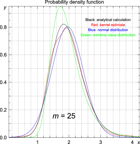
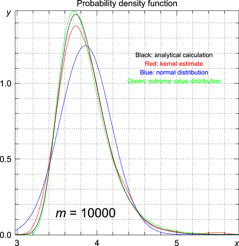
# using the data generated for m = 1
>>> statistics.cpdfc(data, x = 1.96)
[ 0.02511014]
We found 0.025 by fitting a normal distribution, and 0.050 by fitting an extreme value distribution. As

m

increases, the analytically determined tail probability will become more similar to the value estimated from the extreme value distribution, and less similar to the estimate obtained by fitting a normal distribution, as shown in the table below:

$m$	Exact (analytic)	Kernel estimate	Normal distribution	Extreme value distribution
1	0.0250	0.0251	0.0250	0.0497
3	0.0310	0.0310	0.0250	0.0465
5	0.0329	0.0332	0.0250	0.0411
10	0.0352	0.0355	0.0250	0.0451
25	0.0374	0.0377	0.0250	0.0409
100	0.0398	0.0396	0.0250	0.0514
200	0.0405	0.0407	0.0250	0.0482
1000	0.0415	0.0417	0.0250	0.0454
10000	0.0424	0.0427	0.0250	0.0506

4 Installation instructions

In the instructions below, <version> refers to the version number. This software complies with the ANSI-C standard; compilation should therefore be straightforward. First, make sure that Numerical Python (version 1.1.1 or later) is installed on your system. To check your Numerical Python version, type
>>> import numpy; print numpy.version.version
at the Python prompt. To install Statistics for Python, unpack the file:
gunzip statistics-<version>.tar.gz
tar -xvf statistics-<version>.tar
and change to the directory statistics-<version>. From this directory, type
python setup.py config
python setup.py build
python setup.py install
This will configure, compile, and install the library. If the installation was successful, you can remove the directory statistics-<version>. For Python on Windows, a binary installer is available from http://bonsai.ims.u-tokyo.ac.jp/~mdehoon/software/python.

Statistics for Python

Table of Contents

1 Introduction

2 Descriptive statistics

2.1 Univariate descriptive statistics

2.2 Multivariate descriptive statistics

2.2.1 Covariance

2.2.2 Correlation

2.2.3 Linear regression

2.3 Usage

2.3.1 Mean

Arguments

Return values

2.3.2 Median

Arguments

Return values

2.3.3 Variance

Arguments

Return values

2.3.4 Covariance

Arguments

Return values

2.3.5 Correlation

Arguments

Return values

2.3.6 Linear regression

Arguments

Return values

3 Kernel estimation of probability density functions

3.1 Kernel estimation of the density function

3.2 Kernel estimation of the cumulative probability density

3.3 Choosing the bandwidth

3.4 Usage

3.4.1 Estimating the probability density function

Arguments

Return values

3.4.2 Estimating the cumulative probability density function

Arguments

Return values

3.4.3 Estimating the complement of the cumulative probability density function

Arguments

Return values

3.4.4 Calculating the optimal bandwidth

Arguments

Return value

3.5 Examples

3.5.1 Estimating a probability density function

3.5.2 Choosing the kernel and bandwidth

3.5.3 Approaching the extreme value distribution

4 Installation instructions